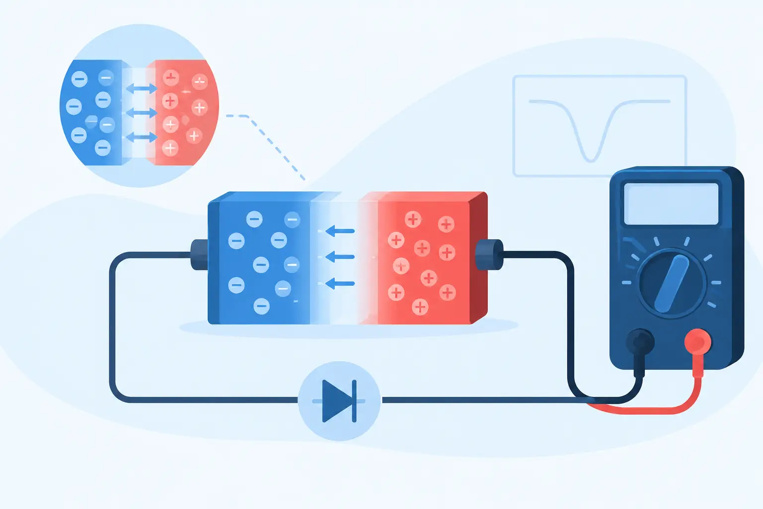
A reverse-biased junction can meet its nominal breakdown specification and still create a system-level problem. In image sensors, low-current analog circuits, power devices, and detector structures, leakage raises noise, shifts bias conditions, and complicates reliability assessment. To calculate junction leakage currents use a model that separates bulk generation, minority-carrier diffusion, perimeter leakage, and field-assisted mechanisms. A single diode saturation-current expression is rarely sufficient.
The required fidelity depends on the design decision. An early process comparison may need only an order-of-magnitude bulk estimate. A leakage specification near the picoampere range, or a device with high fields and complex isolation, requires measured or simulated material parameters, physically correct geometry, and temperature dependence.
How to Calculate Junction Leakage Currents
For a reverse-biased pn junction below avalanche breakdown, begin with the current decomposition:
`I_R = I_gen + I_diff + I_perimeter + I_field + I_parasitic`
Here, `I_gen` is Shockley-Read-Hall generation within the depletion region, `I_diff` is minority-carrier diffusion from the quasi-neutral regions, `I_perimeter` represents surface and edge effects, `I_field` includes trap-assisted tunneling, band-to-band tunneling, and other high-field contributions, and `I_parasitic` covers leakage paths outside the intended junction.
This is an engineering decomposition, not a universal compact-model equation. Its value is diagnostic: each term has a different dependence on reverse bias, area, perimeter, doping, process damage, and temperature. Combining them without identifying their physical origin can produce a numerical answer that is precise but not credible.
Start with depletion width
For an abrupt pn junction, the total depletion width under reverse bias `V_R` is approximately:
`W = sqrt[(2 ε_s / q) (1/N_A + 1/N_D) (V_bi + V_R)]`
where `ε_s` is semiconductor permittivity, `q` is elementary charge, `N_A` and `N_D` are the ionized acceptor and donor concentrations, and `V_bi` is built-in potential. Use consistent units throughout. If concentrations are expressed in cm^-3 and dimensions in cm, the resulting current calculation will be in amperes when the remaining quantities use compatible cgs-based semiconductor units.
In a one-sided junction, the depletion region extends mainly into the lightly doped side. The useful approximation then becomes:
`W ≈ sqrt[2 ε_s (V_bi + V_R) / (q N_light)]`
This relationship explains a common leakage trend. As reverse bias increases, depletion width expands. A wider depleted volume contains more generation centers, so depletion-region leakage normally increases approximately with the square root of reverse voltage before high-field mechanisms become dominant.
Estimate depletion-region generation current
For midgap traps in a reverse-biased silicon junction, a practical first estimate is:
`I_gen = q A n_i W / (2 τ_g)`
where `A` is electrically active junction area, `n_i` is intrinsic carrier concentration, and `τ_g` is the effective generation lifetime. The factor of two assumes a trap near midgap with comparable electron and hole capture behavior. Real defects can depart substantially from this condition, so treat `τ_g` as a calibrated effective parameter unless defect properties are known.
The active area is not automatically the drawn mask area. Guard rings, lateral diffusion, contact overlap, trench isolation, and curved junction boundaries can alter the depleted volume. For a planar test diode, use the measured or process-derived junction area. For a device with lateral field shaping, extract the depleted geometry from the device structure rather than applying a rectangular-area assumption.
Generation lifetime often dominates uncertainty. A value inferred from diffusion length, a clean-wafer lifetime measurement, or a process monitor may not represent the lifetime in a junction that has experienced implantation damage, thermal cycles, etching, passivation, or radiation exposure. When leakage is a critical output, vary `τ_g` across a defensible range instead of presenting one nominal result as a fixed prediction.
Add minority-carrier diffusion current
The ideal diffusion component is commonly written as:
`I_diff = q A n_i^2 [D_n/(L_n N_A) + D_p/(L_p N_D)]`
where `D_n` and `D_p` are electron and hole diffusion coefficients, while `L_n` and `L_p` are the corresponding diffusion lengths. This term is closely related to the reverse saturation current of an ideal diode. It scales with area and with `n_i^2`, making it highly temperature sensitive.
For a well-passivated silicon junction at moderate reverse bias, depletion generation can exceed diffusion current because generation is proportional to `n_i`, while diffusion is proportional to `n_i^2` but is constrained by doping and diffusion lengths. That comparison changes with temperature, doping profile, and lifetime. Do not assume one term dominates without evaluating both.
The abrupt-junction diffusion expression is also a simplification. Graded implants, heterojunctions, incomplete ionization, bandgap narrowing, and high doping require a model that resolves carrier transport and material statistics more completely.
Account for perimeter and surface leakage
Area-based calculations routinely underpredict small-device leakage because the junction edge is not equivalent to the interior. Surface states at the silicon-dielectric interface can provide generation paths, while electric-field crowding near curvature can increase local leakage. A practical measured-model form is:
`I_R = J_A A + J_P P`
where `J_A` is an area leakage density, `J_P` is a perimeter leakage density, and `P` is junction perimeter. By measuring diodes with several area-to-perimeter ratios, an engineer can separate the two coefficients. This approach is especially useful for comparing passivation, guard-ring, and isolation options.
Perimeter fitting does not identify the microscopic mechanism by itself. A large `J_P` may arise from interface generation, etch damage, contamination, incomplete passivation, or local field concentration. It does, however, prevent an area-only model from assigning all measured current to the bulk lifetime.
Check voltage and temperature behavior
Leakage versus reverse voltage is a fast model check. Depletion-generation current should rise as depletion width increases. A sudden upward curvature may indicate edge breakdown, trap-assisted tunneling, or a parasitic path. Once avalanche multiplication begins, the low-field generation and diffusion equations no longer describe total current.
Temperature is equally revealing. Intrinsic carrier concentration changes strongly with temperature, approximately following:
`n_i ∝ T^(3/2) exp[-E_g/(2kT)]`
As a result, diffusion leakage generally has a stronger activated temperature dependence than depletion-region generation leakage. A temperature sweep can therefore help distinguish dominant mechanisms, although trap energies, surface states, and field effects can blur the textbook signatures. Measure at a fixed reverse bias and allow adequate settling time, particularly when dielectric charging or slow traps are present.
Use simulation when the one-dimensional model stops applying
Hand calculations are appropriate for establishing scale, identifying the sensitive parameter, and checking whether a measured result is physically plausible. They become less reliable when doping is two-dimensional, fields crowd around contacts or junction curvature, traps are spatially nonuniform, or the device includes guard rings, trenches, and multiple coupled junctions.
A device simulation should solve Poisson and carrier continuity equations using the process-derived doping distribution. Include Shockley-Read-Hall generation with calibrated trap parameters, concentration-dependent mobility where needed, and field-dependent generation models when the operating field warrants them. The simulation result should still be checked against area, perimeter, voltage, and temperature trends. Numerical detail does not compensate for uncertain trap inputs or an incorrect process profile.
For process-to-device analysis, MicroTec supports two-dimensional process and device modeling, allowing the diffusion profile, junction geometry, and electrical solution to remain connected. That is generally more defensible than transferring a nominal one-dimensional doping value into a leakage calculation for a structure whose current is controlled by a curved edge.
A disciplined calculation workflow
Define the reverse-bias range and operating temperature first. Extract or specify the dopant profiles, active junction geometry, carrier lifetimes, and surface condition. Calculate depletion width, then estimate `I_gen` and `I_diff` separately. If measured data exist, fit area and perimeter contributions before assigning an effective bulk lifetime. Finally, compare predicted voltage and temperature slopes with data and introduce tunneling or avalanche models only when the observed field dependence supports them.
The useful result is not merely a leakage number. It is a statement of which physical mechanism sets that number, which parameter controls its uncertainty, and what process or layout change can reduce it. That distinction turns junction leakage from a late-stage test failure into an engineering variable that can be designed and simulated deliberately.
Leave a Reply