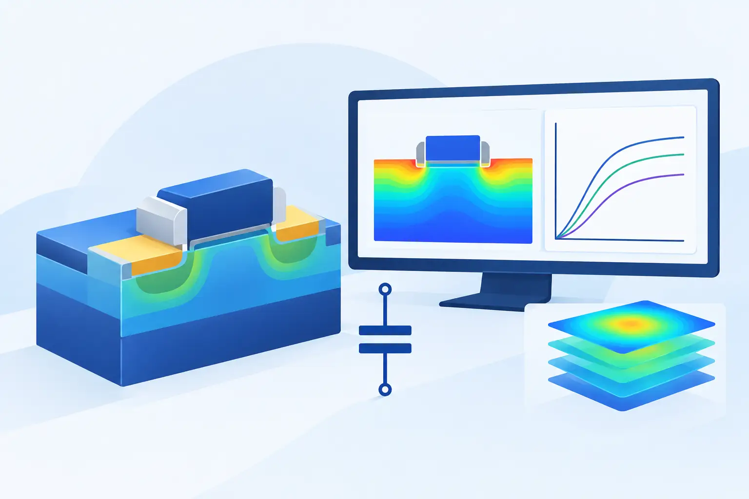
A simulated capacitance curve can look smooth, converge at every bias point, and still be physically wrong. The usual causes are not exotic: an incomplete terminal definition, an inappropriate derivative, insufficient mesh resolution at an interface, or a two-dimensional result reported as though it were a total three-dimensional capacitance. This device capacitance extraction guide sets out a defensible workflow for obtaining capacitance values that can be compared with measurement, compact-model targets, or another numerical solution.
Start with the capacitance definition
Capacitance is not a single quantity for a semiconductor device. The requested result must be tied to a bias condition, terminal configuration, excitation type, and geometry. A MOS capacitor may require high-frequency C-V behavior, quasi-static C-V behavior, or both. A diode may require depletion capacitance under reverse bias. A multi-terminal transistor requires a capacitance matrix, not merely a single value labeled “gate capacitance.”
For an electrostatic or quasi-static extraction, the basic definition is the charge derivative:
[ C_{ij} = frac{partial Q_i}{partial V_j} ]
Here, (Q_i) is the charge assigned to terminal (i), while (V_j) is the voltage applied at terminal (j). The diagonal matrix elements describe the incremental charge response at a terminal to its own voltage. Off-diagonal terms describe coupling between terminals and are commonly negative under a charge-conserving sign convention.
This definition immediately establishes two requirements. First, a capacitance is local to an operating point. A value extracted at zero drain bias may not apply at the intended RF, switching, or breakdown-adjacent bias. Second, every terminal other than the perturbed terminal must have an explicit electrical condition. Floating regions, unspecified substrate contacts, and idealized boundaries can alter field lines and terminal charge substantially.
Choose charge differentiation or small-signal AC analysis
There are two primary extraction routes. Neither is universally superior.
Charge-based differentiation uses a sequence of DC solutions. Sweep the voltage of interest, record terminal charge at each converged point, and compute the numerical derivative. A centered difference is generally preferable away from sweep endpoints:
[ C(V) approx frac{Q(V + Delta V) – Q(V – Delta V)}{2Delta V} ]
This method is direct and makes it easy to inspect the underlying charge curve. It is particularly useful for quasi-static analysis, depletion capacitance, and verification of capacitance-matrix consistency. Its limitation is sensitivity to numerical noise. If the voltage increment is too small, solver tolerances and interpolation error can dominate the difference. If it is too large, the result is an average over a nonlinear part of the C-V curve rather than the desired local derivative.
Small-signal AC analysis linearizes the device equations about a DC operating point and obtains the terminal admittance response at a specified frequency. Capacitance is then inferred from the imaginary component of admittance, with the exact interpretation depending on the terminal configuration and sign convention. This is appropriate when carrier response, traps, series resistance, or frequency dispersion matter. It is not interchangeable with a quasi-static calculation. A high-frequency MOS C-V curve, for example, can differ materially from a low-frequency or quasi-static curve because minority carriers and interface states do not respond on the same timescale.
Use charge differentiation when the engineering question is incremental electrostatic charge at equilibrium or during a slow bias change. Use AC analysis when the question is tied to a measurement frequency or dynamic terminal response. When measured data span frequency, run both where the physical model supports it. The difference is often diagnostic rather than inconvenient.
Build the bias sweep around the device physics
A uniform sweep may be adequate for a simple reverse-biased junction, but it is rarely the most efficient or reliable choice. Refine the bias sampling where depletion width changes rapidly, where inversion begins, near accumulation-to-depletion transition, and around threshold or punch-through behavior. The objective is not to generate a dense plot. It is to resolve the curvature of terminal charge with enough points that the derivative does not depend on arbitrary sweep spacing.
For a MOS structure, begin with a clear definition of substrate bias, gate bias, and any source or drain conditions. For a transistor, hold the non-excited terminals at the intended operating voltages rather than grounding them by habit. Gate-to-channel, gate-to-source, gate-to-drain, and junction capacitances shift as channel charge redistributes with drain bias.
For a pn junction, verify that the contact placement and doping transition represent the fabricated structure. Abrupt-junction theory predicts a useful trend, but graded profiles, diffusion tails, lateral encroachment, and field plates change the effective depletion boundary. A simulated junction capacitance should be treated as a consequence of the solved field and carrier distribution, not as a parameter inserted after the fact.
Terminal charge must be complete and consistently signed
Charge extraction fails when the reported terminal charge excludes a relevant contribution. Depending on the solver and terminal formulation, the extracted quantity may include conduction-related charge, displacement charge, electrode charge, or a combination defined by the numerical formulation. Read the output definition before differentiating it.
The most useful numerical check is charge conservation. For a closed electrostatic system, the sum of electrode and enclosed material charge should be consistent with the applied boundary conditions. In a multi-terminal capacitance matrix, a voltage perturbation should produce terminal-charge changes that satisfy conservation within numerical tolerance. If the matrix does not behave consistently, inspect contact definitions, isolated conductors, dielectric boundaries, and mesh quality before interpreting individual entries.
Sign errors are also common. A simulator may report charge on the metal electrode while an analytical convention is written for charge in the semiconductor. Both can be correct, but their signs differ. Establish the convention once, label it in plots and reports, and preserve it through post-processing.
Mesh where the electric field changes, not everywhere
Capacitance depends on the electric field distribution. A coarse mesh can produce an apparently stable DC potential while under-resolving charge near an oxide interface, junction curvature, contact edge, or narrow dielectric region. Uniformly refining the entire structure is expensive and often unnecessary.
Concentrate mesh refinement at semiconductor-dielectric interfaces, steep doping gradients, depletion boundaries, gate corners, trench edges, and regions where fringing fields terminate. Then perform a mesh-convergence study at representative bias points. Compare extracted capacitance, not only potential or current. A mesh that is adequate for threshold voltage or DC leakage may still be inadequate for overlap or fringe capacitance.
In two-dimensional simulation, report the normalization explicitly. Most 2D device calculations produce capacitance per unit depth, such as F/cm or F/µm, because the third dimension is assumed invariant. Converting that result to total capacitance requires a stated physical width. Do not multiply by a layout dimension unless the cross-section represents the full device width and excludes three-dimensional end effects.
This is a practical boundary between 2D and 3D work. A long, uniform device cross-section can often be modeled efficiently in 2D. Corner effects, finite gate fingers, contact pads, vias, and nonuniform field spreading require a 3D model if they contribute materially to the measured capacitance. Pick the simulator that matches the geometry and governing equations, not a bundle of tools that obscures this choice.
Include the physical models that affect the result
The required physical model set depends on the structure and the quantity being extracted. At minimum, dielectric permittivity, doping-dependent carrier statistics where applicable, and appropriate contact boundary conditions must be credible. For scaled MOS structures, quantum confinement or quantum-potential corrections can alter inversion charge and therefore gate capacitance. Fixed oxide charge and interface charge can shift C-V curves and affect stretch-out.
For measured-frequency comparison, include trap and recombination models only when their parameters are physically supported. Adding poorly constrained traps can make a curve fit one dataset while reducing predictive value elsewhere. The same caution applies to mobility and transport models in transistor capacitance work: use the level of physics required by the terminal response being studied, then validate it against observables that constrain the parameters.
Validate against limits before trusting the curve
A useful extraction should pass simple limiting checks. In a reverse-biased junction, capacitance should generally decline as depletion width expands, absent a geometry-driven exception. In strong accumulation, a MOS capacitor should approach the oxide capacitance expected from dielectric thickness and area, subject to series effects and the selected convention. In depletion, the series combination of oxide and semiconductor depletion capacitance should explain the lower value.
Also compare the integral and differential views of charge. If a small bias perturbation produces a capacitance value that conflicts with the slope of the stored-charge curve, the issue may be sweep spacing, convergence tolerance, or inconsistent charge reporting. Repeat selected points with a smaller voltage step and a refined local mesh. Agreement across these controlled changes is more meaningful than a visually smooth plot.
For multi-terminal devices, inspect reciprocity where the operating conditions and formulation permit it. Differences between corresponding cross-capacitance terms can indicate nonlinearity, terminal-charge allocation effects, or an incomplete numerical convergence. They should be explained, not ignored.
A capacitance result becomes useful when another engineer can reproduce its terminal conditions, geometry normalization, physical model set, mesh basis, derivative method, and validation checks. Treat those items as part of the extracted value, not as background detail. That discipline turns a C-V curve from a presentation graphic into an engineering result that can guide layout, process changes, and compact-model development.
Leave a Reply