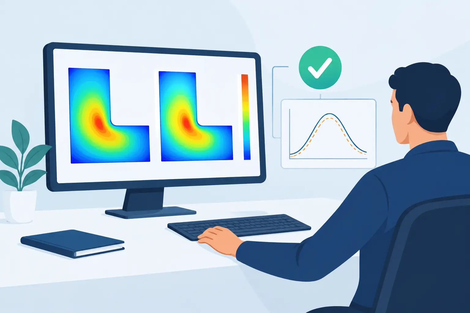
A temperature contour that looks plausible is not evidence that the calculation is correct. To validate numerical heat solver results, an engineer must separate errors caused by the discretization and implementation from errors caused by uncertain material data, boundary conditions, or an incomplete physical model. This distinction matters most in three-dimensional electronic thermal problems, where small errors in interface resistance, power placement, or mesh density can shift predicted junction temperatures enough to change a design decision.
The appropriate validation program depends on the governing equation, the material system, and the decision supported by the model. A steady conduction model for a heat spreader does not require the same evidence as a transient model of a packaged semiconductor with temperature-dependent conductivity. The objective is not to produce a large collection of plots. It is to establish, with traceable tests, that the solver computes the intended physics accurately enough for the engineering question.
Start by separating verification from validation
Verification asks whether the numerical method solves the mathematical equations correctly. Validation asks whether those equations, properties, and boundary conditions represent the physical system. Both are required.
A solver can be verified against an exact solution and still fail to predict a real assembly because the contact resistance or convection coefficient was wrong. Conversely, a carefully measured experiment cannot compensate for a coding error, an under-resolved mesh, or a nonlinear iteration that has not converged. Treat these as separate stages, with separate acceptance criteria.
For a conduction problem, write the model explicitly before testing it. State whether the calculation solves steady or transient heat diffusion, whether thermal conductivity is isotropic or tensor-valued, where volumetric heat generation is applied, and how each external surface is constrained. For transient work, document initial conditions and heat capacity as well. This prevents a common failure mode: comparing a simulation and experiment that do not actually represent the same thermal problem.
Verify the heat equation on problems with known answers
Analytical benchmarks are the fastest way to expose basic errors in assembly, boundary-condition treatment, source integration, and postprocessing. Begin with cases simple enough that the expected temperature field and heat flux are unambiguous.
One-dimensional conduction is not a trivial test
For a slab of thickness L, constant thermal conductivity k, and prescribed temperatures at both faces, the steady temperature profile is linear. With uniform volumetric generation q, the profile becomes quadratic. These cases test more than the final maximum temperature: they reveal whether gradients, flux signs, and source terms are handled correctly.
A composite one-dimensional wall adds material interfaces. The temperature remains continuous across a perfect interface, while the normal heat flux remains conserved. If an interface thermal resistance is present, the temperature must exhibit the corresponding jump. This is a useful test for semiconductor stacks, die attach layers, and multilayer substrates, where material discontinuities are central to the result.
Use a cylindrical or spherical benchmark when the solver will be applied to geometries with radial spreading. Cartesian cases alone may not reveal weaknesses in gradient evaluation or boundary integration on curved surfaces. The selected benchmark should exercise the same features used in production models, not merely the simplest equation the program can solve.
Use manufactured solutions when no convenient benchmark exists
The method of manufactured solutions provides a controlled test for complex three-dimensional domains, variable conductivity, and transient terms. Choose a smooth, known temperature function, substitute it into the governing heat equation, and derive the source term and boundary conditions required to make that function exact.
Because the exact field is known everywhere, errors can be measured in temperature and flux norms as the mesh is refined. This technique is particularly valuable when testing a solver configuration that includes features not available in textbook examples. It can also confirm the expected order of convergence for the chosen spatial discretization, provided the solution is smooth and the nonlinear and linear solvers are converged sufficiently.
Establish mesh independence, not just a fine-looking mesh
A mesh with one million nodes may be appropriate for a detailed package or substrate model, but node count alone says nothing about accuracy. Mesh requirements depend on temperature gradients, geometric aspect ratios, material interfaces, localized heat sources, and the output quantity of interest.
Run at least three systematically refined meshes. Compare the quantities that drive the decision: peak device temperature, average die temperature, heat flow through a boundary, thermal resistance between specified regions, or the time to reach a temperature limit. A visually similar contour field is not enough. If peak temperature changes materially between the two finest meshes, the result is not mesh independent.
Refine locally where physics demands it. Thin dielectrics, metal traces, narrow heat sources, vias, sharp corners, and high-resistance interfaces often require substantially smaller elements than bulk regions. Excessive uniform refinement can make a calculation expensive while leaving the governing local error unresolved.
When the numerical formulation supports it, estimate observed convergence from successive mesh solutions. Such estimates must be interpreted carefully. Singular corners, discontinuous material properties, and idealized point or line sources can reduce the apparent convergence rate. In those cases, the practical question is whether the engineering output has stabilized under physically defensible local refinement.
Check energy conservation on every serious model
For steady-state conduction, total heat leaving the domain must equal total generated heat, within a tolerance consistent with the solver settings and numerical precision. For a model with prescribed heat fluxes, convection, and fixed-temperature boundaries, calculate each contribution independently and confirm the balance.
This check is simple and unusually powerful. A model may display a smooth temperature field while losing energy through an incorrectly assigned boundary, a sign convention error, or an incomplete source region. In transient calculations, account for stored thermal energy as well as boundary heat flow and internal generation over each time interval.
Energy balance should be reported as a residual relative to the total applied power, not only as an absolute value. A residual of 0.01 W may be insignificant in a 100 W model and unacceptable in a 20 mW device calculation. For coupled electrothermal problems, also confirm that electrical power dissipation is transferred consistently to the thermal source term.
Demonstrate solver convergence separately from mesh convergence
Mesh convergence does not prove that each individual solution is converged. Iterative linear solvers, nonlinear conductivity models, radiation boundaries, and temperature-dependent sources introduce algebraic error that can contaminate a refinement study.
Track the residual definition used by the solver and relate it to physical outputs. A small equation residual is necessary, but it is not always sufficient. Tighten the linear and nonlinear tolerances and observe whether peak temperature, boundary heat flow, and thermal resistance change. If they do, the original solver tolerance was inadequate for the requested output.
Time-dependent models require an equivalent time-step study. Reduce the time step while holding the spatial mesh fixed, then determine whether transient peaks, phase lags, and integrated energy change. Implicit time integration can remain stable at large time steps while still smoothing a physically important temperature excursion.
Validate against measurements with an uncertainty budget
Experimental comparison is the final test of model adequacy, but measurements must be interpreted with the same discipline applied to the numerical solution. A thermocouple attached to a package surface, an infrared image, and an electrical junction-temperature estimate do not measure the same quantity or have the same spatial and temporal resolution.
Define the comparison location, averaging area, and time reference precisely. If an infrared measurement averages over several pixels while the simulation reports a nodal maximum, disagreement may be caused by mismatched observables rather than incorrect physics. Map the simulation result onto the measurement definition before calculating error.
An uncertainty budget should include power dissipation, thermal conductivity, layer thickness, contact resistance, ambient conditions, sensor placement, calibration, and boundary-condition estimates. In many assemblies, interface resistance and convection uncertainty dominate the discrepancy. It is reasonable to calibrate an uncertain parameter when independent measurements constrain it, but do not tune several parameters until the model matches one data set. That produces a fitted result, not a predictive model.
Validate under more than one operating condition. A model calibrated at a single power level or airflow condition may conceal compensating errors. Agreement across multiple powers, boundary conditions, or package orientations is stronger evidence that the thermal model represents the relevant mechanisms.
Match the test plan to the model’s intended use
A solver used to rank heat-spreader layouts may need reliable relative temperature differences more than an exact absolute junction temperature. A model used for reliability assessment may require tighter confidence in local peaks and transient cycling. State the required accuracy before validation begins, because the required mesh, material characterization, and measurement effort follow from that decision.
For large three-dimensional problems, a dedicated numerical tool such as SibLin can make the calculation practical, but no software package removes the need for a documented verification and validation workflow. The appropriate solver is the one that matches the equation set, geometry, and mesh scale without adding tools the project does not require.
The most useful thermal simulation is not the one with the most detailed contour plot. It is the one for which an engineer can explain the governing assumptions, quantify numerical sensitivity, account for energy, and state clearly where measured evidence supports the prediction.
Leave a Reply