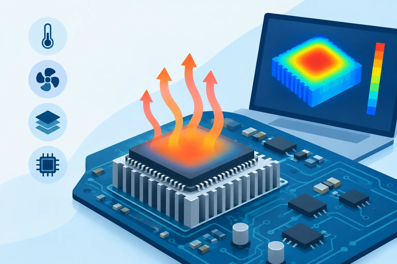
A temperature map is only useful if it explains the engineering decision in front of you. For a device engineer, that may mean locating a localized hot spot before it changes mobility or accelerates degradation. For a package or interconnect researcher, it may mean separating a genuine spreading-resistance effect from an artifact of mesh design. Thermal solvers are the numerical engine behind those decisions, but their value depends on how well their physics, geometry, boundary conditions, and numerical method match the problem.
What thermal solvers actually solve
At their core, thermal solvers calculate the temperature field in a structure by enforcing conservation of energy. In steady-state form, the governing equation is commonly written as:
`∇ · (k∇T) + Q = 0`
Here, `T` is temperature, `k` is thermal conductivity, and `Q` represents volumetric heat generation. Transient analysis adds heat storage through density and specific heat. The equation is compact; the engineering problem is not. Conductivity may vary by material, temperature, crystal orientation, or layer. Heat generation may be concentrated in a small active region. Interfaces, contacts, convection boundaries, and fixed-temperature surfaces can dominate the result.
A useful solver does more than produce a colored contour plot. It should resolve gradients where the physics demands resolution, preserve numerical stability on practical meshes, and allow the engineer to test whether the result changes when assumptions are refined. The relevant question is not whether a solver can calculate temperature. Nearly every thermal code can do that for a simple block. The question is whether it can calculate the right temperature distribution for the actual electronic structure under study.
Why electronic thermal problems are rarely simple
Semiconductor and electronic assemblies combine sharply different length scales. A heat-generating region may be measured in microns, while the substrate, package, heat spreader, or surrounding domain is orders of magnitude larger. A mesh that is sufficiently fine everywhere can become prohibitively expensive. A mesh that is too coarse near a source, interface, or narrow current path can flatten the very gradient that determines the design outcome.
Material contrast creates another difficulty. Silicon, dielectrics, metals, adhesives, and ambient regions conduct heat differently. In thin multilayer structures, thermal resistance may be governed less by the bulk material than by a poorly represented interface or an assumed boundary condition. Treating a contact as perfectly isothermal, for example, can make a predicted peak temperature look reassuringly low while concealing a bottleneck in the real structure.
Heat is also coupled to other device behavior. Joule heating depends on current distribution. Carrier transport and mobility can change with temperature. In power devices, electrothermal feedback may concentrate dissipation where the local temperature has already risen. In these cases, a thermal solution is not necessarily the end of the analysis. It may need to be coupled to Poisson, diffusion, drift-current, or spreading-resistance equations.
Selecting thermal solvers by problem dimension
The first selection decision is usually dimensionality. A two-dimensional thermal model is appropriate when the geometry and heat flow are effectively invariant along one axis, or when it is being used early in device development to examine cross-sectional behavior. It can be fast, transparent, and highly useful for comparing process or layout alternatives.
A three-dimensional model is required when lateral heat spreading, finite contact geometry, nonuniform sources, or asymmetric boundary conditions determine the result. This is common in real packages, resistor networks, sensor structures, power devices, and layered electronic assemblies. A 2D model may estimate vertical heat flow correctly yet miss a lateral path that either relieves or intensifies a local hot spot.
Neither approach is inherently superior. The practical choice depends on what must be resolved. Starting in 2D is often sensible when establishing material parameters, source profiles, and boundary assumptions. Moving to 3D becomes necessary when the omitted dimension changes the resistance network or local temperature maximum. Engineers should avoid treating a lower-dimensional model as a final answer simply because it runs quickly, but they should also avoid using a large 3D mesh where a validated 2D representation answers the question directly.
Mesh capacity is not the same as mesh quality
Large problems require large meshes, but node count alone does not establish credibility. A million-node model can still be wrong if critical interfaces are under-resolved or if the outer boundary is placed too close to the heat source. Conversely, a smaller mesh can provide an excellent answer when it is concentrated around steep gradients and paired with physically justified boundaries.
Mesh-convergence testing remains one of the most effective checks. Refine the regions around active devices, narrow conductors, material transitions, and peak-temperature locations. Then compare the quantities that drive the decision: maximum temperature, temperature difference across an interface, heat flux through a boundary, or equivalent thermal resistance. If those quantities move materially with refinement, the model has not yet earned confidence.
The numerical formulation matters as well. Thermal solvers should remain stable across irregular geometries and substantial conductivity variation, without forcing the user into excessive manual tuning. For research and industrial design work, the preferred tool is one that can solve the required mesh while leaving time for sensitivity studies. A single expensive run is less valuable than a workflow that permits engineers to test the assumptions behind it.
Boundary conditions deserve the same scrutiny as equations
Many thermal simulations fail quietly at the boundary. A fixed-temperature boundary is convenient, but it represents a perfect heat sink at a prescribed location. Convection conditions require a heat-transfer coefficient and ambient temperature, both of which may be uncertain. Adiabatic boundaries can be appropriate at planes of symmetry, but not as a default method for reducing model size.
The boundary should represent the physical test or operating environment. If a device is mounted to a temperature-controlled chuck, a fixed-temperature boundary may be justified at the chuck interface. If heat leaves through air or liquid cooling, convection and radiation may need consideration. If the model terminates within a substrate or package, the analyst should establish that the truncation boundary is far enough away not to distort the thermal field.
A disciplined approach is to run sensitivity cases. Vary the convection coefficient, interface resistance, source power, or sink temperature within credible ranges. The resulting spread in peak temperature may be more useful to a design review than a single value reported to an unrealistic number of decimal places.
Coupled physics changes the tool requirement
A thermal-only calculation is suitable when power dissipation is known and does not change appreciably with temperature. That assumption is often reasonable for a prescribed resistor, a fixed heat source, or an initial package study. It becomes weaker when current crowding, temperature-dependent conductivity, or semiconductor transport affects where power is generated.
For coupled problems, the solver must support a consistent treatment of the relevant equations and variables. Heat generation should arise from the electrical solution where appropriate, and temperature should feed back into material parameters when the physics requires it. This adds computational cost and modeling responsibility, but it can be essential for predicting hot spots, failure margins, and nonuniform device behavior.
This is also where standalone tools can be advantageous. An engineer investigating a 3D heat-transfer or spreading-resistance problem does not necessarily need a broad software suite designed for unrelated workflows. Siborg Systems’ SibLin, for example, is designed for three-dimensional numerical problems involving heat transfer alongside Poisson, diffusion, drift-current, and spreading-resistance equations, including meshes exceeding 1,000,000 nodes. The appropriate choice remains problem-specific: select the simulator that matches the governing physics and geometry, not a bundle that adds complexity without analytical value.
A practical verification sequence
Before accepting a thermal result, establish the intended use of the model. Is it screening alternatives, correlating with measurement, estimating a safe operating limit, or supplying temperature data to an electrical calculation? The required level of geometric detail follows from that purpose.
Next, check energy balance. The heat entering or generated within the domain should be consistent with heat leaving through its boundaries, within the expected numerical tolerance. Review the temperature field for nonphysical discontinuities, unexpected extrema, and gradients that align suspiciously with coarse mesh transitions rather than material features.
Then compare against an independent reference whenever one exists. This may be an analytical resistance estimate, a simplified one-dimensional calculation, a measured thermal resistance, or a known limiting case. Agreement does not prove every model assumption, but disagreement often identifies where the model needs attention.
Finally, document the inputs that matter: material properties, source definition, interface treatment, boundary conditions, mesh strategy, convergence behavior, and sensitivity results. Thermal simulation becomes much more valuable when another engineer can understand why the result is credible and what operating range it supports.
A well-chosen thermal model should leave the engineering team with a decision they can defend: where heat is generated, how it escapes, which assumption controls the uncertainty, and what design change is most likely to improve the result.
Leave a Reply