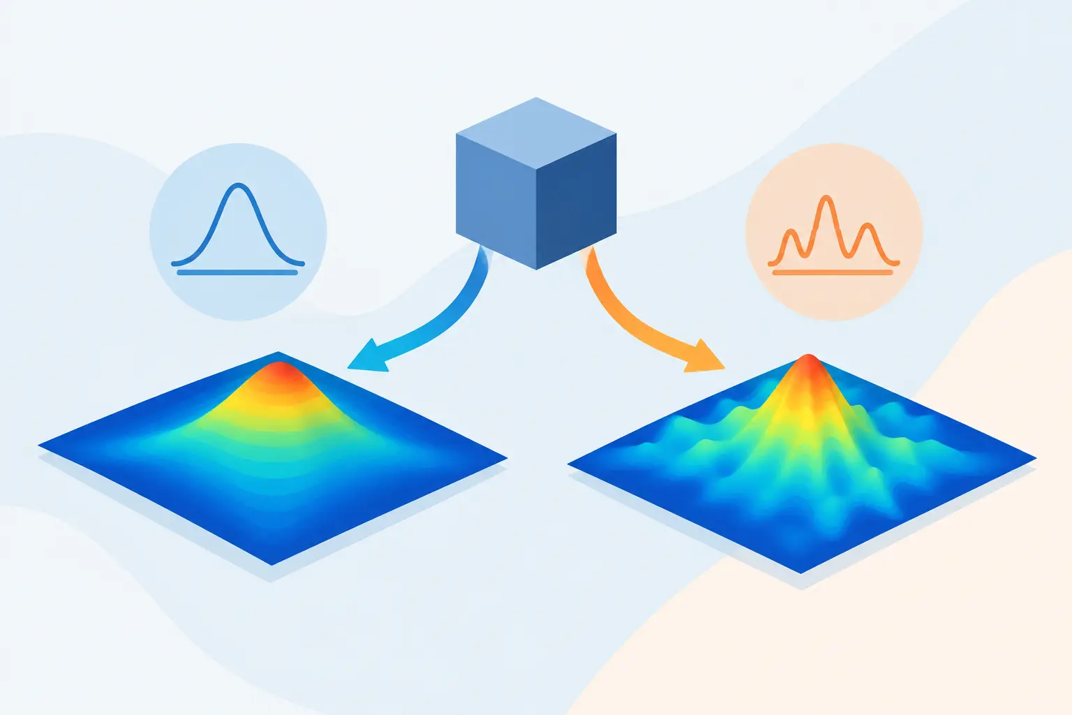
A residual that falls for several iterations, stalls, and then grows is not merely a failed run. It is diagnostic evidence. Understanding why solvers diverge requires separating a numerical failure from a model that is physically inconsistent, poorly scaled, or being asked to resolve features the mesh and algorithm cannot support.
For semiconductor, electrothermal, diffusion, and field calculations, divergence usually arises from an interaction rather than a single setting. A sharp doping transition affects the electric field; the electric field changes carrier transport; temperature changes mobility; and each update changes the coefficients seen by the next solve. The larger and less well-scaled those changes become, the harder the nonlinear iteration must work to find a self-consistent state.
Why Solvers Diverge in Coupled Physical Models
A numerical solver diverges when its successive iterates move away from a solution, or fail to make sufficient progress toward one. In practice, this may appear as an increasing residual norm, oscillating terminal currents, nonphysical negative concentrations, repeated linear-solver failure, or a time-step controller that reduces the step until the simulation can no longer advance.
These symptoms are related but not identical. A linear solver can fail because the matrix is ill-conditioned, even when the nonlinear formulation is sound. A nonlinear solver can oscillate because the update is too large, even when every linear subproblem is solved accurately. A transient calculation can reject time steps because a real physical transition is occurring faster than the selected temporal resolution.
The first question is therefore not, “Which tolerance should be relaxed?” It is, “At what level does the calculation first fail?” Residual histories, iteration counts, matrix diagnostics, and field plots provide more useful answers than a single final error message.
Strong nonlinear feedback
Poisson, continuity, drift-current, diffusion, and heat-transfer equations are often coupled through coefficients that depend on the unknown solution. Conductivity can depend on temperature, carrier density can depend exponentially on potential, and recombination terms can change rapidly across a depletion region.
Newton-type methods assume that a local linear approximation is useful for the next correction. When the initial state is far from the solution, or when material properties change sharply over one update, that assumption can fail. The result is an overshoot: the next iterate lands in a region where the equations have very different behavior, and subsequent corrections alternate or grow.
This is common when bias is applied in one large increment, when a high-power thermal source is enabled abruptly, or when a simulation begins from a uniform initial condition that bears little resemblance to the expected device state. The issue is not that nonlinear methods are unsuitable. It is that their convergence region is finite.
Mesh resolution and mesh quality
A mesh must resolve the shortest physical length scale that materially affects the result. In device simulation, that may be a junction, an oxide interface, a contact edge, a high-field region, or a narrow current path. In thermal analysis, it may be a thin layer, a heat-source boundary, or a constriction that drives spreading resistance.
An under-resolved gradient can produce a solution that is inaccurate yet apparently converged. It can also cause divergence when the discretization generates large local coefficient changes or nonphysical oscillations. Excessive refinement, however, is not automatically safer. It increases matrix size, can worsen conditioning when adjacent elements differ greatly in size, and may expose weak scaling in the formulation.
Element shape matters as much as element count. Highly skewed cells, abrupt aspect-ratio changes, and poor transitions between fine and coarse regions can degrade the discrete operator. A million-node model with controlled grading is generally easier to solve than a smaller model containing a few severely distorted regions.
Scaling and conditioning
Physical simulations naturally combine quantities with very different magnitudes and units. Potential may be measured in volts, carrier density in inverse cubic centimeters, heat generation in watts per cubic meter, and thermal conductivity over a wide material-dependent range. If equations and unknowns are not scaled appropriately, the matrix can contain coefficients separated by many orders of magnitude.
Poor scaling does not necessarily make a model incorrect. It makes numerical decisions less reliable. A stopping criterion that is reasonable for one equation may be meaningless for another. Pivoting, preconditioning, and iterative linear solves may all lose effectiveness as the condition number grows.
This problem often appears after adding a physically valid feature: a highly conductive contact, a nearly insulating layer, extreme doping, or a large material-property contrast. The feature is not the mistake. It may simply require a formulation, mesh, and solver configuration that account for the resulting scale separation.
Boundary conditions and source definitions
Many divergence problems begin at the boundary. Conflicting Dirichlet conditions, an omitted reference potential, an unintended insulated surface, or a source applied over the wrong region can make the discrete system singular or physically implausible.
Check units with equal care. A heat source entered as a total power when the model expects volumetric generation can drive temperatures far beyond the intended range. A concentration specified in meters rather than centimeters can alter transport coefficients by orders of magnitude. Numerical divergence is sometimes the first visible symptom of a dimensional error.
A Disciplined Diagnosis Sequence
The fastest path is usually to reduce uncertainty, not to change every available solver parameter. Start by saving the failing case and making one controlled modification at a time.
Establish the failure signature
Determine whether failure occurs on the first nonlinear iteration, after several corrections, only after mesh refinement, or only beyond a particular bias, power, or time. Record the residual for each equation separately where possible. A rising Poisson residual suggests a different problem from a stable Poisson solve paired with failing continuity equations.
Also inspect the last valid solution. Peak field, temperature, carrier concentration, and current-density plots often reveal the location where the model becomes unreasonable. A localized spike near a contact or interface points toward mesh, boundary, or material-definition issues. A global oscillation more often indicates nonlinear update control or inadequate scaling.
Verify a simpler physical case
Remove coupling strategically. Solve electrostatics before transport, conduction before temperature-dependent conductivity, or diffusion before adding drift terms. Use constant properties temporarily if they are otherwise strongly temperature or field dependent.
This is not a substitute for the final model. It identifies the first added mechanism that changes a convergent problem into a failing one. Once isolated, that mechanism can be reintroduced through continuation rather than as a full-strength discontinuity.
Use continuation rather than a single jump
Continuation is one of the most effective remedies for nonlinear divergence. Ramp voltage, current, optical generation, heat load, or a material parameter over a series of smaller solves. Each converged state becomes the initial estimate for the next one.
The appropriate increment depends on the physics. A smooth low-field device may tolerate substantial voltage steps. Breakdown, self-heating, phase-sensitive material behavior, or strongly activated transport may require much smaller increments near the transition. Adaptive stepping is useful, but it should be reviewed rather than accepted blindly. A sequence of tiny steps can hide a problematic model region while consuming substantial computation time.
Examine the mesh where physics changes fastest
Refine locally around junctions, interfaces, contacts, and narrow thermal paths. Then compare results against a second, systematically modified mesh. If peak values change materially while integrated current, total power, or terminal resistance remain stable, the issue may be local resolution. If global quantities also change erratically, inspect mesh grading and boundary definitions before adding more nodes.
For a three-dimensional calculation in SibLin, this distinction matters especially as models approach or exceed 1,000,000 mesh nodes. Large node counts justify careful control of mesh quality and solver settings; they do not compensate for a poorly posed boundary-value problem.
Corrective Actions That Match the Failure
When nonlinear updates overshoot, apply damping or reduce the continuation increment. Damping trades iteration speed for a larger convergence region. It is often appropriate near sharp transitions, although excessive damping can make routine cases unnecessarily slow.
When the linear system is poorly conditioned, review variable and equation scaling, material contrasts, and mesh grading. Select preconditioning and linear-solver controls appropriate to the matrix structure rather than tightening nonlinear tolerances first. A nonlinear method cannot compensate for an inaccurately solved linear correction.
When a transient calculation repeatedly rejects steps, reduce the maximum time step near the event and inspect whether source discontinuities can be ramped. Verify that the selected temporal scheme matches the required balance between stability and accuracy. A very stable method may suppress numerical growth while smearing a fast physical response; a less dissipative method may require tighter step control.
When fields or concentrations become nonphysical, investigate constraints, constitutive models, and boundary data before increasing iteration limits. More iterations can make an incorrect formulation converge more convincingly. The goal is a credible solution to the stated equations, not simply a residual below a threshold.
A useful final practice is to retain a converged baseline for every significant model. Change geometry, mesh, material data, boundary conditions, and solver controls in identifiable increments. When a run fails, the most informative next calculation is usually the smallest one that can prove which new assumption changed the behavior.
Leave a Reply