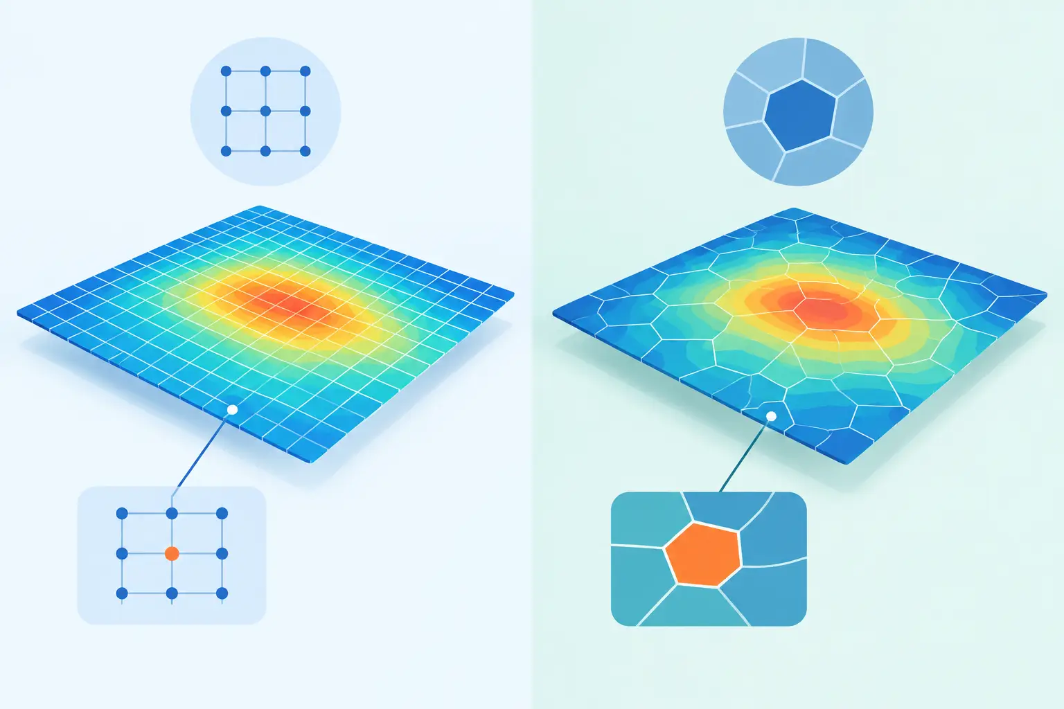
A discretization method is not a minor implementation choice when the model includes steep dopant gradients, heterogeneous thermal conductivity, current crowding, or material interfaces. In finite difference vs finite volume comparisons, the useful question is not which method is universally better. It is which formulation preserves the physical quantities, geometry, and boundary behavior that control the result.
For semiconductor process, device, electrostatic, and thermal work, both methods can produce accurate solutions. Both convert partial differential equations into algebraic systems that a numerical solver can evaluate on a mesh. Their differences appear in how they represent derivatives, enforce conservation, accommodate geometry, and expose errors near interfaces and boundaries.
Finite Difference vs Finite Volume: The Core Distinction
The finite difference method starts from a differential equation at discrete points. Derivatives are replaced with difference expressions formed from neighboring nodal values. For a one-dimensional diffusion equation, for example, a second derivative can be represented by the familiar difference between values at adjacent nodes and the center node, divided by the square of grid spacing.
This pointwise approach is direct and efficient on structured Cartesian meshes. When the geometry is rectangular or can be represented cleanly with a mapped grid, finite differences produce compact stencils and matrices with predictable sparsity. That is attractive for Poisson, diffusion, and heat-transfer equations over regular device regions.
The finite volume method begins differently. It integrates the governing conservation law over a small control volume. Fluxes through the faces of that volume are then approximated, and the net flux is balanced against sources or storage within the volume. The resulting equation is associated with a cell rather than simply with a mathematical point.
That construction gives finite volume a defining property: local conservation. If flux leaves one control volume through a shared face, an equal and opposite flux enters the neighboring volume. For mass, charge, energy, or momentum balance, this is more than an aesthetic advantage. It can determine whether an integrated physical quantity remains credible as the mesh is refined or operating conditions change.
Where Finite Differences Are Often the Better Fit
Finite difference methods are particularly effective when the domain is structured, the governing equations are smooth within each region, and computational efficiency matters. A rectangular silicon cross-section, a layered thermal stack approximated on an orthogonal mesh, or a regular three-dimensional field problem can be handled with simple stencils and well-understood boundary treatments.
The method also aligns naturally with many educational and research workflows. Engineers can inspect a stencil, verify its order of accuracy, and relate each matrix coefficient to a neighboring node. This transparency is useful when debugging convergence problems or testing a new physical model.
For elliptic equations such as Poisson’s equation, finite differences can be highly accurate and economical on uniform or smoothly graded meshes. Grid refinement is straightforward. High-order derivative approximations are also relatively accessible when the solution is sufficiently smooth and the boundaries do not dominate the error.
The limitations become more visible around irregular geometry and abrupt material changes. A staircase representation of a curved boundary may be acceptable for a coarse preliminary model but can distort electric fields or heat flow near the actual surface. At semiconductor interfaces, a naive difference approximation can also mishandle discontinuous coefficients unless the flux formulation and interface conditions are treated carefully.
Finite difference does not inherently mean nonconservative. A finite difference scheme written in flux form can preserve a discrete conservation balance. The distinction is that conservation is built into the finite volume derivation, while it must be deliberately retained in a finite difference formulation.
Where Finite Volume Has an Advantage
Finite volume methods are a natural choice when conservation across material boundaries is central to the engineering decision. Consider heat conduction through regions with sharply different thermal conductivities. The physically relevant quantity at an interface is heat flux continuity, not merely a smooth numerical temperature curve. A face-flux formulation makes that requirement explicit.
The same logic applies to diffusion and carrier transport. If a model represents generation, recombination, injection, or current flow between regions, a cell-based balance helps ensure that what is lost from one region appears in another or is accounted for by a source term. This is especially valuable when the mesh is nonuniform and gradients are concentrated in a small portion of the domain.
Finite volume also handles complex geometry more naturally when paired with unstructured meshes or body-fitted control volumes. Curved package features, angled heat spreaders, nonrectangular contacts, and irregular material regions can be represented without forcing every boundary onto an orthogonal grid.
That flexibility has costs. Face interpolation, gradient reconstruction, and nonorthogonal corrections introduce additional numerical choices. A poorly constructed finite volume scheme can be diffusive, unstable, or only first-order accurate in areas where the mesh is strongly skewed. Conservation alone does not guarantee an accurate local solution.
Interfaces, Boundary Conditions, and Mesh Quality
For semiconductor and thermal simulation, the choice often turns on interfaces rather than on the governing equation’s name. Poisson’s equation, for example, can be solved well by either approach. The relevant questions are whether permittivity changes abruptly, whether interfaces are aligned to the mesh, whether surface charge is present, and whether electrode boundaries contain corners or thin features.
In a finite difference model, aligned planar interfaces can be treated accurately using appropriate coefficient averaging and matching conditions. On an orthogonal mesh, this can be computationally efficient and physically sound. When interfaces cut obliquely through cells, the formulation requires more care.
In finite volume, discontinuous properties are commonly placed at cell faces through a flux calculation. Harmonic averaging of conductivity-like coefficients is often appropriate for transport normal to layered interfaces, while arithmetic averaging may be incorrect in that setting. The correct choice follows the physical flux law and mesh arrangement, not a generic numerical preference.
Boundary conditions deserve the same scrutiny. Dirichlet conditions specify a field value, such as a fixed potential or temperature. Neumann conditions specify flux. Robin conditions combine both, as in convective thermal boundaries. Each can be implemented by either method, but the numerical location of the boundary and the treatment of half-cells or ghost nodes influence accuracy. A solver that converges tightly can still converge to a biased result if the boundary model is misplaced.
Accuracy Is Not Just a Formal Order
It is tempting to compare a second-order finite difference scheme with a first- or second-order finite volume scheme and choose based on formal truncation error. That comparison is incomplete. Formal order describes behavior as mesh spacing approaches zero under assumptions about smoothness and mesh quality. Device-scale and package-scale problems often violate those assumptions near corners, junctions, contacts, and discontinuous material properties.
A lower-order conservative method on a mesh that resolves the relevant interface can outperform a nominally higher-order method applied to a poorly represented geometry. Conversely, a structured finite difference mesh with efficient local refinement may be the better engineering choice for a domain that is fundamentally layered and orthogonal.
The practical test is mesh convergence against the outputs that matter: peak temperature, junction location, total current, voltage drop, thermal resistance, or spreading resistance. Monitor integral balances as well as local extrema. If refinement changes a critical result materially, the discretization error remains part of the answer.
Solver Behavior and Computational Cost
Both methods commonly lead to large sparse linear or nonlinear systems. The discretization affects the matrix structure, which in turn affects memory use and the performance of direct or iterative solvers.
Finite differences on structured grids usually produce regular stencil patterns that are favorable for efficient storage and multigrid-style methods. Finite volume matrices can remain sparse and well behaved, but irregular connectivity and nonorthogonal corrections may increase assembly cost and make preconditioning more consequential.
For three-dimensional models with hundreds of thousands or more than one million mesh nodes, the governing issue is rarely the method name alone. Mesh topology, equation coupling, nonlinear material models, solver tolerances, and available memory can dominate runtime. Select the numerical approach based on the complete workload, not on a claim that one discretization is always faster.
A Practical Selection Rule
Start with the physics and geometry. Finite differences are often the efficient choice for structured domains, smooth fields, and problems where regular-grid accuracy and compact implementation are priorities. Finite volume is often preferable when strict local balance, irregular geometry, or flux continuity across complex interfaces drives the result.
Then verify the implementation. Ask whether material discontinuities use physically appropriate face coefficients, whether boundary conditions are imposed at the correct geometric location, and whether the solver reports meaningful convergence measures. Residual reduction alone is not enough. Conservation error and mesh-refinement behavior should be checked against the quantities used to make the engineering decision.
The best discretization is the one that makes the physical model easier to verify. If a structured finite difference mesh represents the device faithfully, it may be the most economical and transparent solution. If the problem is governed by face fluxes through irregular regions, a finite volume formulation may reduce risk where it matters most: in the result used to design, qualify, or reject the device.
Leave a Reply