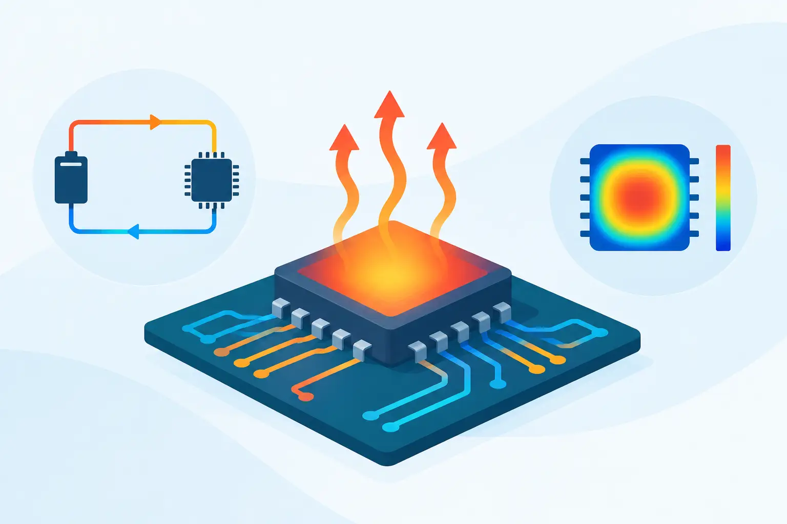
A power MOSFET can meet its room-temperature electrical specification and still fail in the field because one localized region carries slightly more current, heats faster, and becomes still more conductive. That feedback loop is the practical reason electrothermal coupling examples matter. Electrical and thermal behavior cannot be treated as separate post-processing steps when temperature changes carrier transport, resistivity, leakage, contact behavior, or breakdown margin.
For semiconductor devices, interconnects, and electronic packages, coupling is not merely the addition of a heat equation to an electrical model. It is a bidirectional calculation. Current density produces heat through Joule dissipation and, where applicable, recombination or other physical mechanisms. The resulting temperature field changes the electrical parameters that determined the current distribution in the first place. Whether this interaction is stabilizing or destructive depends on the material system, bias condition, geometry, thermal boundary conditions, and time scale.
What Electrothermal Coupling Solves
The electrical side of a coupled problem commonly includes Poisson, carrier continuity, drift-current, or conduction equations. The thermal side solves heat transfer with internally generated power. These equations are linked through material properties and source terms. Electrical conductivity, carrier mobility, saturation velocity, intrinsic carrier concentration, thermal conductivity, and contact resistance may all vary with temperature.
A decoupled workflow can still be appropriate when dissipated power is low, temperature rise is demonstrably small, or the goal is a first-pass design estimate. It becomes inadequate when a local hot spot changes the current path, when leakage rises strongly with temperature, or when thermal spreading is governed by three-dimensional package and substrate geometry.
The practical question is therefore not whether temperature exists in the device. It always does. The question is whether the calculated temperature field changes electrical operation enough to alter a design decision.
Electrothermal Coupling Examples That Expose Risk
Current crowding in power devices
Consider a lateral or vertical power transistor operating near its rated current. A small nonuniformity in cell geometry, metallization, or substrate resistance can produce a locally higher current density. The local power density, approximately J·E, increases temperature. In many operating regimes, a temperature increase reduces carrier mobility and raises on-resistance, which can redistribute current away from the hot region. That is a potentially stabilizing response.
The behavior is not universally benign. In other devices and bias ranges, temperature-driven changes in threshold voltage, leakage, or conductivity increase local current. The hot region then receives more power and the solution can evolve toward current filamentation or thermal runaway. A simulation must resolve both the local electrical field and the heat-spreading path to distinguish these cases. A spatially averaged junction temperature cannot reveal whether one small region has exceeded a reliability limit.
Self-heating in SOI and RF transistors
Silicon-on-insulator structures are a familiar self-heating case. The buried oxide provides electrical isolation but has much lower thermal conductivity than bulk silicon. Heat generated near the channel encounters a restricted path to the substrate, increasing channel temperature during sustained bias.
The electrical effects can include reduced mobility, transconductance compression, shifted threshold behavior, and altered output characteristics. For analog and RF operation, these changes influence gain, linearity, and bias stability rather than only maximum current. The relevant time scale also matters. A short pulse may see a different thermal impedance and electrical response than continuous-wave operation, even at identical peak power.
Interconnect heating and electromigration drivers
Metal interconnect analysis often begins with a current-density limit, but current density alone does not establish reliability. Local resistive heating raises conductor temperature, and metal resistivity generally rises with temperature. Higher resistivity increases local Joule heating, particularly at vias, line-width transitions, corners, and contacts where current crowds.
This interaction affects electromigration assessment because atomic transport is strongly temperature dependent. A model that predicts acceptable average line temperature can still miss a high-temperature via region that shortens lifetime. Three-dimensional modeling becomes valuable when heat is shared among neighboring lines, dielectric layers, metal stacks, and the substrate. The thermal path is rarely one-dimensional in a real layout.
Leakage-driven heating in reverse-biased structures
Reverse-biased diodes, detector structures, and high-voltage junctions provide another important example. Leakage current frequently has a strong temperature dependence. A local defect, edge field enhancement, or imperfect guard structure can initiate leakage. The associated dissipation raises temperature, which can raise leakage further.
The resulting feedback may remain modest and settle at a higher operating temperature, or it may approach thermal runaway if heat removal is limited. Accurate analysis requires the reverse-bias electric field, local generation mechanisms, and thermal boundary conditions to be represented consistently. Treating leakage as a fixed room-temperature current removes the very mechanism under investigation.
Spreading resistance in contacts and substrates
Spreading resistance is inherently an electrothermal problem when appreciable current passes through a finite contact area. Current entering a semiconductor, conductive film, or substrate does not spread uniformly at the contact edge. The resulting concentration of current density causes localized power generation, while the same geometry restricts heat flow away from that region.
This is especially relevant for probes, high-current contacts, semiconductor test structures, and compact devices with small source or drain areas. A two-dimensional cross-section may adequately represent a long, uniform structure. A circular contact, irregular pad, or localized heat source generally requires a three-dimensional model. The choice should follow the dominant geometry, not software convenience.
Modeling Choices That Determine the Result
Coupled simulation is only as credible as its physical assumptions. Material-property data should cover the expected temperature range, rather than relying on a single nominal value. Thermal boundary conditions also require care. A fixed-temperature boundary may represent a well-controlled heat sink, but it can be overly optimistic for a die attached through multiple interfaces. Thermal contact resistance, convection assumptions, and package layers can dominate the predicted junction temperature.
Mesh refinement should follow gradients, not visual symmetry. Refine near junctions, contact edges, narrow conductive paths, dielectric bottlenecks, and anticipated hot spots. A coarse mesh may conserve total power while smearing the peak temperature enough to produce a misleading reliability conclusion. Conversely, indiscriminate refinement can create an unnecessarily expensive problem. The engineering objective is convergence of the quantities that drive a decision: peak temperature, current crowding, voltage drop, or location of maximum field.
Numerical coupling strategy also matters. A fully coupled solution can be necessary where feedback is strong or where the system is near instability. Iterative electrical and thermal solves may be sufficient for weaker coupling, provided the iterations converge and the solution is checked against mesh and tolerance changes. There is no virtue in solving a larger system than the physics requires, but there is clear risk in using a one-way thermal correction where electrical behavior is temperature-sensitive.
Matching Dimensionality to the Engineering Question
A two-dimensional simulation remains efficient for process cross-sections, planar junction behavior, and devices that are uniform along one direction. It can establish diffusion profiles, junction placement, electric-field distributions, and first-order self-heating trends with far less computational cost than a full three-dimensional model.
Three-dimensional analysis is warranted when lateral heat spreading, finite contacts, nonuniform metallization, multiple heat sources, or package-level paths control the result. SibLin v1.2 is intended for this class of numerical workload, solving three-dimensional heat transfer alongside Poisson, diffusion, drift-current, and spreading-resistance problems on meshes exceeding 1,000,000 nodes. The useful distinction is straightforward: use the dimensionality required by the heat and current paths, not the dimensionality that produces the quickest plot.
From Simulation Output to a Design Decision
The most useful electrothermal result is not a temperature contour by itself. It is an explanation of which geometric feature, material parameter, or boundary condition controls the margin. If a hot spot is driven by a narrow metal transition, widening that transition may be more effective than changing the global heat sink. If the limiting effect is substrate spreading resistance, a contact-layout change may outperform a thicker top metal layer.
Results should be examined across bias, ambient temperature, and realistic cooling assumptions. A design that is acceptable at nominal voltage can become marginal during startup, pulsed overload, or elevated ambient operation. Comparing peak temperature alone is also insufficient when device performance depends on temperature-induced voltage shift, leakage, or current redistribution.
Electrothermal analysis earns its place when it converts a suspected failure mechanism into a specific, testable design change. The right model is the one that identifies where power is generated, where heat is trapped, and how that temperature rise changes the electrical state that created it.
Leave a Reply