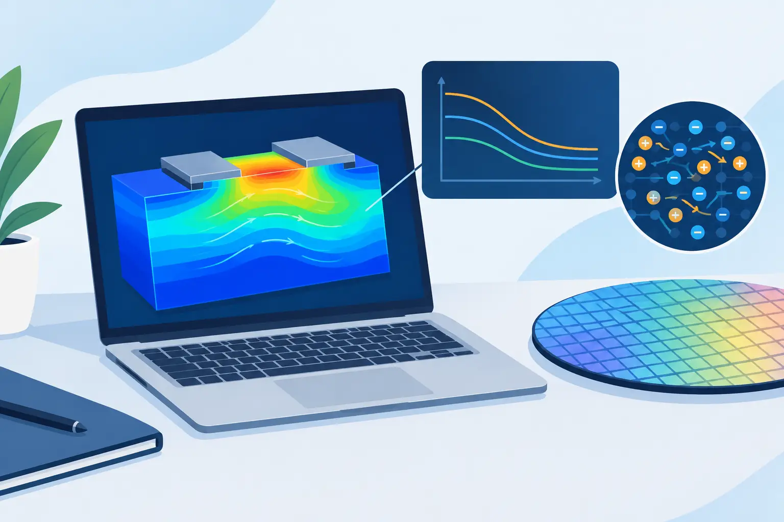
A carrier mobility modeling guide is most useful when it starts with the measurement or device behavior that must be reproduced, not with a menu of mobility equations. Mobility affects drive current, sheet resistance, transconductance, channel-field response, diffusion current, and self-heating predictions. A model that is adequate for a low-field silicon resistor can be inadequate for a short-channel MOSFET, a high-voltage drift region, or a heterostructure.
The practical objective is not to select the most elaborate model available. It is to select a model whose physical assumptions match the material system, doping range, temperature range, field regime, and transport quantity under study. Extra parameters without relevant calibration data can make a simulation less defensible, not more accurate.
Define the mobility problem before selecting a model
Carrier mobility describes how readily electrons or holes move under an electric field. In device simulation, mobility is not generally a material constant. It changes with temperature, ionized impurity concentration, carrier concentration, crystal orientation, mechanical stress, electric field, and scattering mechanisms. The appropriate representation therefore depends on what limits transport in the device.
Begin by separating the observable of interest from the physical mechanism likely to control it. For example, a measured resistivity profile in a doped silicon layer is commonly sensitive to concentration-dependent mobility and incomplete ionization. MOSFET on-current is additionally sensitive to transverse-field degradation near the semiconductor-insulator interface and velocity saturation along the channel. A power device may require credible high-field transport throughout a lightly doped drift region, while an elevated-temperature study may depend primarily on phonon scattering and temperature scaling.
This definition should also state whether the result is local or terminal-level. A local mobility contour can appear plausible while the simulated contact resistance, drain current, or breakdown behavior remains incorrect. Terminal characteristics, extracted sheet resistance, Hall mobility, and measured temperature coefficients provide stronger calibration targets because they constrain the model in the context of the full structure.
Establish a defensible baseline mobility model
For many silicon process and device problems, the baseline is a low-field, doping-dependent mobility relation for electrons and holes. Such a relation represents the reduction in mobility caused by ionized impurity scattering as dopant concentration increases. It is usually the first mobility dependency needed when simulating diffused resistors, source and drain regions, junctions, and other structures with substantial doping variation.
The baseline must be evaluated with the rest of the physical model set. Dopant activation, incomplete ionization, bandgap narrowing, carrier statistics, and recombination assumptions can all change the calculated carrier concentration. Since mobility depends on the relevant concentration variable, an apparent mobility error may originate in the ionization or statistics model instead.
Use measured data at the same temperature and, where possible, the same material quality and doping species. Published bulk curves are useful reference points, but they may not represent implanted layers, polycrystalline films, strained channels, or material systems with defects and interface effects. A parameter fit should not silently compensate for process damage or contact resistance that has not been modeled elsewhere.
Check concentration definitions and units
Mobility expressions may use total dopant concentration, ionized impurity concentration, majority carrier concentration, or a combined concentration term. These alternatives are not interchangeable at low temperature, under incomplete ionization, or in compensated material. Confirm the definition implemented by the simulator before comparing coefficients from a paper or a process-design kit.
Unit errors remain a common source of misleading results. Concentrations expressed in cm^-3, electric fields in V/cm, and mobilities in cm^2/V-s must be consistent with the solver’s input conventions. A fit that appears unusually successful over one bias range may simply contain a hidden unit conversion error that will fail when extrapolated.
Add field dependence only when the device requires it
At sufficiently high lateral electric field, drift velocity no longer increases linearly with field. A high-field or velocity-saturation model is then needed for short-channel transistors, high-voltage structures, and other regions where carrier velocity approaches a limiting value. Applying this correction to every problem without checking field levels adds complexity with little benefit.
The critical question is whether the device result is controlled by high-field transport. In a long resistor operated at modest bias, a velocity-saturation model should have limited influence. In a transistor channel, the same model can materially change current saturation, output conductance, and transient behavior. Compare the simulated field distribution with the model’s transition range rather than inferring relevance from applied voltage alone. A small applied voltage across a very short distance can create a large field.
Field-dependent mobility also requires numerical care. Strong feedback exists between electric field, carrier density, mobility, current density, and local potential. Abrupt mesh transitions or poorly resolved depletion regions can introduce field peaks that are numerical artifacts. Refine the mesh where field gradients, junction curvature, interfaces, or narrow channels determine the result. Mesh refinement should reduce changes in the extracted current or resistance to an acceptable engineering tolerance.
Treat surface, temperature, and stress effects separately
Bulk mobility is not channel mobility. Near an oxide-semiconductor interface, transverse field, surface roughness, interface charge, and scattering can reduce carrier mobility substantially. For MOS structures, use a surface or transverse-field correction when the simulation goal includes inversion-layer current, threshold-region transconductance, or mobility extraction. Calibrate it against relevant electrical data, such as effective mobility or current-voltage curves, rather than relying only on bulk material tables.
Temperature dependence should be included whenever the operating range is broad, self-heating is significant, or the device is intended for thermal environments. Phonon scattering generally lowers mobility as temperature rises, while impurity scattering can produce a different trend. The resulting mobility-temperature behavior may not be monotonic across all doping levels. A model calibrated only at 300 K should not be assumed valid across a thermal cycle.
Stress and crystallographic orientation are similarly conditional. They matter when the process intentionally uses strained material, when orientation-dependent transport is part of the design, or when mechanical stress materially alters channel performance. If those effects are outside the device specification and no calibration data exist, adding them can create a false impression of physical precision.
Couple mobility to the transport formulation
Mobility modeling cannot be assessed independently from the transport equations. In drift-diffusion simulation, mobility converts electric field into drift current and contributes to diffusion through the Einstein relationship, subject to the statistics formulation used. In high-field conditions, energy-balance or hydrodynamic transport may be more appropriate when carrier heating and nonlocal effects affect the measured behavior.
Drift-diffusion remains efficient and useful for many process and device analyses, particularly when calibration is based on DC characteristics and dimensions are not dominated by nonlocal transport. It may be insufficient for aggressively scaled channels or fast transient conditions where carriers do not equilibrate locally with the field. The correct choice depends on the question being asked and the experimental evidence available, not on a preference for a more computationally expensive formulation.
For electrothermal work, mobility must also be coupled consistently to lattice temperature and power dissipation. A calculation that changes mobility with temperature but does not resolve the relevant thermal path may predict an internally inconsistent current reduction. Conversely, a thermal solution requires enough electrical fidelity to calculate where heat is generated. Three-dimensional thermal spreading can be decisive when contacts, metallization, and asymmetric layouts control local temperature.
Calibrate in a controlled sequence
Calibration is most effective when each step has a clear target. Start with equilibrium or low-bias measurements to establish doping, activation, and low-field mobility. Then fit field-dependent behavior using output characteristics, velocity-related data, or suitable high-bias measurements. Add surface mobility corrections for MOS channel data, and finally validate the temperature dependence against measurements at multiple temperatures.
Avoid changing several mobility parameters at once. If a simulated current improves after simultaneous adjustments to doping, interface charge, saturation velocity, and contact resistance, the result does not identify the physical cause. Preserve a record of parameter values, data sources, temperature, geometry, mesh settings, and extraction method. This record is essential when the model is later applied to a revised process or layout.
A credible calibration should be tested outside the fitting condition. For example, a model fitted to a single gate voltage should be checked across gate bias, drain bias, temperature, and device dimensions when those ranges matter to the design. Agreement at one operating point is a fit. Agreement across independent conditions is evidence that the physical assumptions are useful.
Numerical checks that protect the result
Mobility models can conceal numerical weaknesses because they directly influence the current equation. Before accepting a result, check mesh convergence, bias-step convergence, current continuity, and sensitivity to boundary conditions. Inspect spatial plots of electric field, carrier density, mobility, current density, and temperature together. An isolated spike in one quantity often explains an unexpected terminal characteristic.
Also distinguish physical parameter uncertainty from solver error. If reasonable changes in a mobility coefficient alter drain current by 10 percent, reporting four significant figures in the final current adds no value. Sensitivity analysis identifies which mobility inputs deserve better measurements and which are not decision-critical.
MicroTec is suited to two-dimensional semiconductor process and device studies where diffusion profiles, Poisson solutions, and drift-current behavior must be evaluated without assembling an unnecessary software bundle. For problems in which three-dimensional heat flow or spreading resistance governs the electrical response, the mobility model should be assessed alongside the thermal solution rather than treated as a separate correction.
The useful stopping point is not the most detailed carrier mobility model. It is the point at which the selected physics, calibration data, mesh, and transport formulation support the engineering decision with known limits.
Leave a Reply