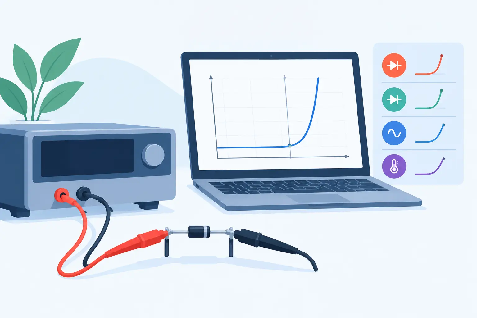
A diode I-V sweep can look satisfactory on a semilog plot while still producing misleading saturation current, ideality factor, series resistance, or shunt resistance values. To extract diode IV parameters that remain useful outside a single curve fit, the measurement range, chosen model, and physical interpretation must agree. The task is not simply to obtain the smallest residual. It is to identify which transport mechanism dominates each part of the curve and fit only where the assumptions are valid.
For process and device engineers, this distinction matters directly. Extracted parameters are often used to compare lots, diagnose contact degradation, calibrate simulation models, or establish whether a change in diffusion, implantation, anneal, or metallization altered device behavior. A parameter set that compensates for measurement artifacts or an incomplete model can obscure the actual process change.
Start with a diode model that matches the data
The baseline forward-current model is the Shockley diode equation:
[ I = I_S left[expleft(frac{qV_D}{nkT}right)-1right] ]
where (I_S) is the saturation current, (n) is the ideality factor, (V_D) is the voltage across the junction, (q) is the elementary charge, (k) is Boltzmann’s constant, and (T) is absolute temperature. For an ideal diffusion-controlled junction, (n) approaches 1. Recombination within the depletion region commonly produces a region with (n) closer to 2.
Measured devices rarely follow this equation across the full voltage range. A more useful engineering representation includes series and parallel paths:
[ I = I_S left[expleft(frac{V – IR_S}{nV_T}right)-1right] + frac{V – IR_S}{R_{SH}} ]
Here, (R_S) represents bulk, spreading, contact, and interconnect resistance, while (R_{SH}) represents junction leakage or another parallel conduction path. This equation is implicit in current, so numerical solution or nonlinear regression is normally required for a global fit.
The correct model depends on the device and voltage range. A low-current detector diode, power rectifier, Schottky diode, solar cell, and small-area PN test structure can all require different treatment. Adding every possible correction term may reduce residual error, but it also creates poorly identifiable parameters. Use the simplest model that explains repeatable physical behavior.
Measure before you fit
Parameter extraction begins with a defensible I-V measurement. Record the device temperature, probe configuration, compliance settings, sweep direction, settling time, voltage step size, and current range. These details determine whether the apparent curve represents the junction or the test setup.
At low currents, instrument offset, cable leakage, light exposure, humidity, and surface contamination can dominate. At high currents, self-heating and voltage drop in leads or probe contacts can make the diode appear more resistive than it is. For small devices, probe-contact repeatability can be a significant fraction of the extracted series resistance.
Use four-terminal sensing when the device layout permits it, particularly when series resistance is an extraction target. Measure forward and reverse sweeps where hysteresis, trapping, or thermal lag is plausible. A sweep that changes shape with direction or rate should not be reduced to a single static parameter set without further investigation.
Current polarity also requires attention. For semilog analysis, use the magnitude of the forward current only after confirming that the sign convention and offset correction are physically consistent. Taking a logarithm of noisy values near zero current can manufacture a false slope.
Establish the useful voltage regions
A typical measured curve has at least three regions. The low-current region may be governed by leakage, recombination, or instrumentation limits. A middle forward-bias region may approximate exponential behavior and is the usual source of (n) and (I_S). At high current, series resistance bends the semilog trace and eventually dominates the differential resistance.
Do not choose a fitting window because it looks linear by eye. Calculate the local slope, inspect residuals, and compare repeated sweeps. If the inferred ideality factor changes steadily throughout the supposed exponential region, the data may contain more than one transport mechanism, an uncorrected series-resistance effect, or temperature drift.
Extract diode IV parameters from local behavior
For a region where series resistance and shunt current are negligible, rearrange the diode equation as:
[ ln(I) = ln(I_S) + frac{V}{nV_T} ]
A linear regression of (ln(I)) against (V) provides a first estimate. If the fitted slope is (m), then:
[ n = frac{1}{mV_T} ]
and the intercept gives (I_S). At 300 K, (V_T = kT/q) is approximately 25.85 mV. This approach is transparent and useful, but only inside a verified exponential region. Applying it to the full forward curve generally overestimates the ideality factor because series resistance reduces the slope at higher current.
For series resistance, inspect the differential resistance:
[ frac{dV}{dI} approx R_S + frac{nV_T}{I} ]
At sufficiently high forward current, the (nV_T/I) term decreases and the differential resistance approaches (R_S). Numerical differentiation amplifies noise, so smooth the data cautiously or fit a physically constrained model to the raw I-V points. Excessive smoothing can erase a real transition between recombination and diffusion current.
Estimate shunt resistance from the low-bias slope when the parallel-current term dominates:
[ R_{SH} approx left(frac{dI}{dV}right)^{-1} ]
This estimate is most credible when taken near zero bias under controlled dark conditions. Reverse-bias leakage is related but not automatically equivalent to a constant shunt resistance. Trap-assisted generation, edge leakage, breakdown precursors, and surface conduction may each produce voltage-dependent current.
Use global fitting as verification, not a substitute for physics
Once local estimates are available, fit the complete selected data range to the series-resistance and shunt-resistance model. Initialize the optimizer with values obtained from the exponential, low-bias, and high-current regions. Constrain parameters to physically meaningful ranges, such as positive resistances and positive saturation current.
Weighting matters. Ordinary least squares on linear current gives disproportionate importance to the largest-current points. Fitting logarithmic current can overemphasize the low-current region and becomes unreliable near zero or where current changes sign. A weighted residual based on measured uncertainty, or a fit performed separately in physically distinct regions, is often more defensible than one unweighted global regression.
Examine parameter correlation before treating results as process indicators. In a limited voltage range, (I_S), (n), and (R_S) can compensate for one another. A narrow confidence interval reported by an optimizer does not prove that the model is uniquely identified. Repeat measurements across temperature, area, and device geometry provide stronger evidence.
Temperature-dependent data are especially valuable. A physically meaningful saturation current should exhibit a consistent temperature trend, while the ideality factor and leakage mechanisms may reveal transitions that are invisible at one temperature. Area scaling can similarly separate perimeter leakage from bulk junction behavior.
Connect extraction to device and process analysis
A parameter is useful when it points to a plausible physical cause. An increase in (R_S) may indicate a contact, metallization, spreading-resistance, or substrate issue. A change in (R_{SH}) may suggest junction damage, contamination, edge termination weakness, or a surface-passivation problem. A shift in ideality factor can reflect recombination, interface states, barrier inhomogeneity, or an extraction window that no longer isolates the same mechanism.
For simulation calibration, do not force a two-dimensional device model to reproduce every measurement artifact. Use extracted values to define targets for junction behavior, contact resistance, doping profiles, and leakage mechanisms that are supported by the physical model. MicroTec can then evaluate how process conditions and device geometry affect the quantities behind the fitted parameters rather than merely reproducing a curve shape.
Report enough information to reproduce the result
A useful extraction record states the device geometry, temperature, measurement configuration, voltage and current ranges, selected fitting window, model equation, weighting method, and parameter uncertainty. Include the measured curve and residuals, not only the final values. If a parameter came from a local approximation rather than a global fit, say so directly.
The most reliable diode parameters are not those produced by the most elaborate optimizer. They are the values that remain stable when the measurement is repeated, the fitting region is justified, and the result agrees with known device physics.
Leave a Reply