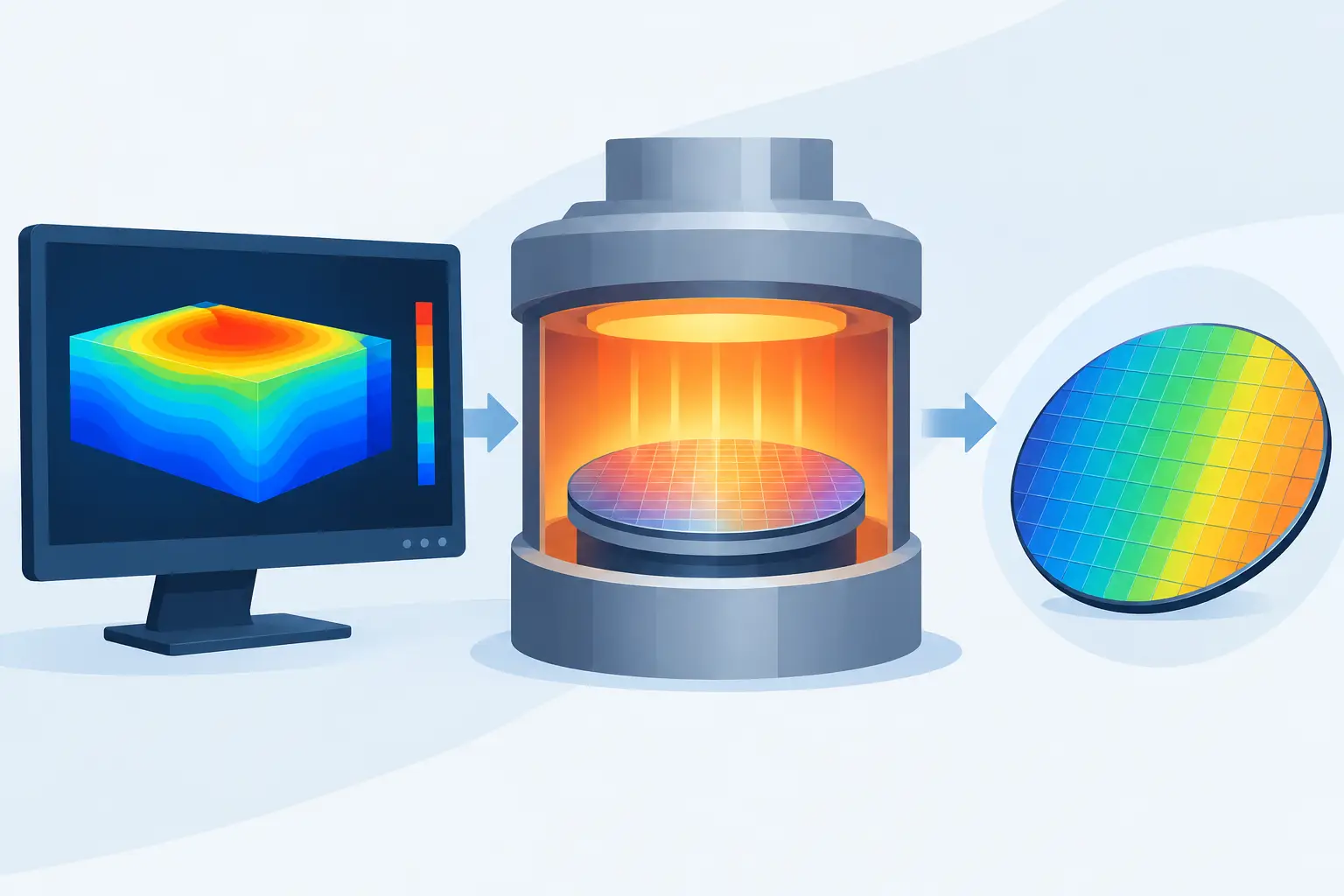
An anneal step can determine whether an implanted junction meets its sheet-resistance target, preserves a shallow profile, or diffuses far enough to compromise short-channel control. That is why learning how to simulate wafer annealing starts with the process objective, not with selecting a temperature from a furnace recipe. The simulation must represent the thermal history and the mechanisms that redistribute and electrically activate dopants during that history.
For most process studies, wafer annealing is not an isolated calculation. It follows implantation, deposition, oxidation, or a preceding diffusion step, and its result becomes the starting profile for later etches, implants, or device simulation. A credible model therefore carries the wafer structure and impurity distributions forward through the full relevant sequence.
Define the anneal result before building the model
Start by specifying the quantity that will be used to judge the run. A junction depth extracted at a stated concentration, sheet resistance, active dopant dose, peak concentration, or lateral encroachment can each be valid targets. They do not necessarily respond to the same model assumptions in the same way.
For example, a drive-in anneal after a deep implant may be evaluated primarily by vertical junction depth. A rapid thermal anneal for a source-drain extension is more sensitive to transient diffusion, activation, and the steepness of the near-surface profile. If the anneal is part of a bipolar or power-device flow, the relevant question may instead be whether a long thermal budget moves dopant across a buried interface or alters a collector profile.
This distinction matters because a model calibrated only to junction depth can still produce an incorrect sheet resistance. Electrical activity depends on more than total chemical concentration. It can be affected by clustering, precipitation, compensation, and the local defect population.
Build the correct pre-anneal wafer state
The anneal calculation is only as useful as its initial condition. Construct the substrate, epitaxial layers, deposited films, oxide regions, and implanted regions that exist immediately before heat treatment. Preserve material boundaries because they can change diffusion behavior and serve as sources or sinks for point defects.
For implanted wafers, use an implantation model that establishes a physically reasonable as-implanted profile, including lateral distribution when geometry makes it relevant. Dose and energy alone are not sufficient if the application depends on channeling tails, screen oxide effects, tilt, rotation, or masking topology. A one-dimensional approximation may be acceptable for a blanket implant far from pattern edges; it is usually not sufficient for a patterned shallow junction.
The inputs that should be documented for every anneal run include:
- wafer orientation, substrate type, background dopant, and starting concentration
- implant species, dose, energy, tilt, rotation, and any screen or sacrificial oxide
- layer materials and thicknesses present during the thermal step
- furnace or rapid-thermal temperature history, including ramps and holds
- ambient conditions, especially when oxidation or nitridation occurs during annealing
The objective is traceability. When a measured profile and a simulated profile disagree, an engineer should be able to separate uncertainty in the implant condition from uncertainty in the diffusion or activation model.
Represent the thermal budget, not just peak temperature
A nominal anneal temperature is an incomplete process description. Diffusion depends strongly on temperature, so time spent in the ramp can be material for short, high-temperature recipes. Two cycles with the same peak temperature and dwell time can produce different profiles when their ramp rates differ substantially.
Define the complete temperature-time sequence: ramp-up, stabilization if applicable, main soak, ramp-down, and any separate preheat or post-anneal cycle. For conventional furnace diffusion, the soak commonly dominates the thermal budget. For spike and rapid thermal anneals, ramp segments may account for a meaningful fraction of dopant motion and defect evolution.
Use measured or equipment-qualified temperature profiles when they are available. A recipe setpoint is not always the wafer temperature, particularly during fast transients or with differing wafer emissivity and chamber loading. If the purpose of the study is process-window prediction, run credible upper and lower thermal-budget cases rather than treating one nominal profile as exact.
Ambient must also be explicit. An oxidizing ambient can inject interstitials and grow oxide, changing the near-surface diffusion behavior of some dopants. An inert anneal may preserve a different defect balance. Treating these cases as identical can give a numerically clean result that does not describe the actual wafer process.
Select diffusion and activation physics to match the regime
The simplest diffusion treatment uses concentration-dependent diffusivity. It may be suitable for long, moderate-dose drive-in steps where empirical calibration data supports the approximation. It is not automatically adequate for high-dose implants or modern thermal cycles.
Ion implantation creates excess vacancies and interstitials. During subsequent annealing, their evolution can cause transient enhanced diffusion, particularly for dopants whose transport couples strongly to point defects. At high concentrations, clustering and incomplete activation can limit the electrically active fraction even when the chemical dose is unchanged. Interfaces, oxidation, and damage-removal kinetics further affect the result.
Choose the least complex physics set that addresses the measured behavior and intended decision. Adding mechanisms without calibration can create more adjustable parameters than useful predictive power. Conversely, omitting transient diffusion or activation in a shallow-junction study can force an engineer to compensate with unrealistic diffusivity values.
A practical calibration sequence is to first match the as-implanted profile, then match a limited set of annealed chemical profiles, and finally compare electrical observables such as sheet resistance or spreading-resistance data. Keep the calibration set independent from the experiments used to evaluate prediction. Otherwise, agreement may only show that the model has been fitted to the same data.
Use mesh refinement where gradients and interfaces demand it
Annealing simulations solve coupled transport behavior across concentration gradients that can be steep near the surface, at junctions, and around mask or spacer edges. Mesh resolution should be concentrated in those regions rather than distributed uniformly across a large substrate depth.
In two-dimensional process simulation, refine the mesh around implant windows, oxide-silicon interfaces, shallow junctions, and locations where lateral diffusion affects device dimensions. Extend the domain deeply enough that the lower boundary does not influence the region of interest. A boundary placed too near a diffusing profile can artificially retain or remove dopant, depending on its condition.
Perform a mesh-convergence check before trusting extracted values. Reduce local cell size and compare junction depth, peak active concentration, sheet resistance, and lateral spread. If these outputs shift materially with refinement, the original grid was not adequate. The best mesh is not the finest possible mesh; it is the coarsest mesh that produces stable engineering outputs within the required tolerance.
Validate outputs against measurements that answer different questions
Plotting concentration versus depth is necessary, but it is not sufficient. Compare the simulated chemical and active profiles separately when data permits. Secondary-ion mass spectrometry measures chemical concentration, while sheet resistance, electrochemical capacitance-voltage methods, or spreading-resistance measurements provide different evidence about activation and electrically relevant profiles.
When comparing junction depth, state the concentration criterion and whether it refers to total or active dopant. When comparing sheet resistance, ensure that carrier mobility and compensation assumptions are consistent with the extracted quantity. A close match to one measurement can conceal an error in another.
Sensitivity analysis is especially useful near a process limit. Vary dose, peak temperature, dwell time, ramp rate, and selected model parameters within credible uncertainty bands. If a small temperature change produces a large junction-depth shift, the process is thermally sensitive and simulation should report a range, not only a nominal value.
Choose the dimensionality that matches the question
A vertical blanket diffusion can often be studied efficiently in one dimension during early calibration. Once mask edges, spacers, isolation regions, or neighboring implants affect the outcome, use a two-dimensional process model. The extra dimension is justified when lateral diffusion changes an electrically important length or overlap.
MicroTec v4.23 is suited to this two-dimensional process and device workflow, allowing engineers to carry process-defined dopant profiles into later electrical analysis without purchasing an unnecessary software bundle. For thermal problems that require full three-dimensional heat-transfer analysis, the thermal field should be established with a tool designed for that dimensionality before simplifying it into an appropriate process thermal history.
Treat anneal simulation as a controlled engineering model
The useful deliverable is not a color contour of dopant concentration. It is a documented model that states the starting structure, thermal cycle, physical assumptions, mesh criteria, calibration evidence, and extracted metrics. That record allows another engineer to reproduce the result, challenge an assumption, or apply the model to a nearby process condition.
Wafer annealing is sensitive to details that are easy to omit: a few seconds of ramp time, an oxidizing ambient, a damaged implant tail, or a boundary placed too close to the active region. Account for the details that control the decision, calibrate against more than one observable, and let the required process tolerance determine how much model complexity is justified.
Leave a Reply